Decision Tree In Machine Learning
A Python Mache learning decision tree is evaluated and examples are provided to aid in understanding. A decision tree is one of the most powerful and popular tools for classification and prediction.
Decision trees are flowchart-like trees in which each internal node identifies a test on an attribute, each branch represents the result and each leaf node (terminal node) identifies the class.
Python Decision Tree
We’ll show you how to create a “Decision Tree“. You can use a decision tree as a tool to help you make decisions based on your previous experiences.
As an example, a person may decide whether or not to attend a music concert.
We are fortunate that the example person registered every time there was a music concert in the town. As well, he/she has added any information they have about the singer.
| Singer Age | Singer Experience | Rank | Concert Region | Go |
| 26 | 5 | 8 | CA | YES |
| 32 | 2 | 2 | USA | NO |
| 40 | 10 | 7 | N | NO |
| 28 | 6 | 3 | USA | YES |
| 19 | 1 | 9 | USA | YES |
| 43 | 3 | 4 | CA | NO |
| 33 | 7 | 6 | N | YES |
| 55 | 15 | 8 | CA | YES |
| 63 | 20 | 9 | N | YES |
| 59 | 7 | 8 | N | YES |
| 22 | 2 | 9 | USA | NO |
| 29 | 6 | 2 | CA | YES |
| 31 | 3 | 8 | USA | YES |
| 62 | 5 | 4 | CA | No |
| 47 | 8 | 7 | USA | YES |
The Python program can now build a decision tree using this data set, which can help determine whether or not attending new music concerts is worth it.
How it Works?
In order to read the dataset with pandas, first import the required modules:
The data set should be read and printed as follows:
Example
All data must be numerical when making a decision tree.
Concert Region and Go are not numerical columns, so we need to convert them into numerical ones.
Map() in Pandas takes a dictionary containing information about how values should be converted.
{'CA': 0, 'USA': 1, 'N': 2}
‘CA’ becomes 0, ‘USA’ becomes 1, and ‘N’ becomes 2.
Numerical values can be converted from string values as follows:
Example
After that, we need to separate the target column from the feature column.
Our target column is the column with the predicted values, while the feature columns are the columns we try to predict from.
A feature column is varx and a target column is vary:
Example
Our decision tree can now be created according to the details we supplied, and we can save it as a .png file:
Save the Decision Tree as an image and show it:
Example
Result Explained
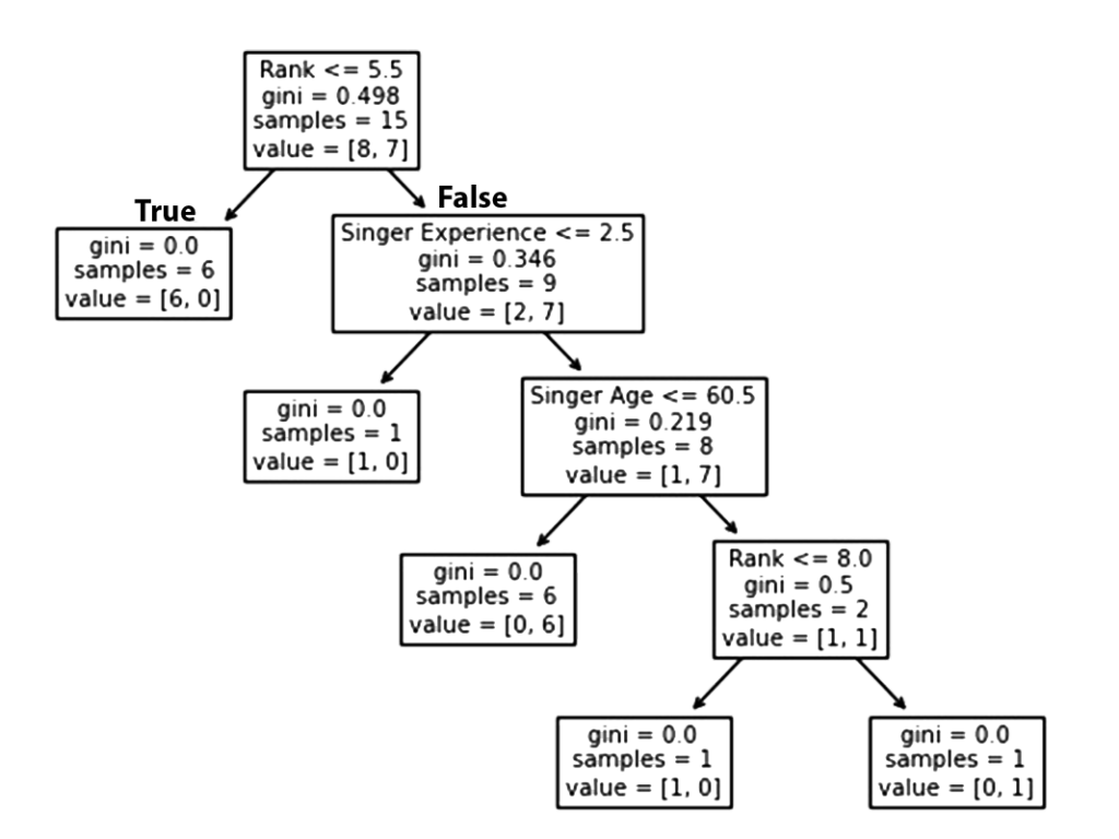
By analyzing your previous decisions, the decision tree calculates your likelihood of attending a particular singer’s concert or Not.
Here are the different aspects of the decision tree:
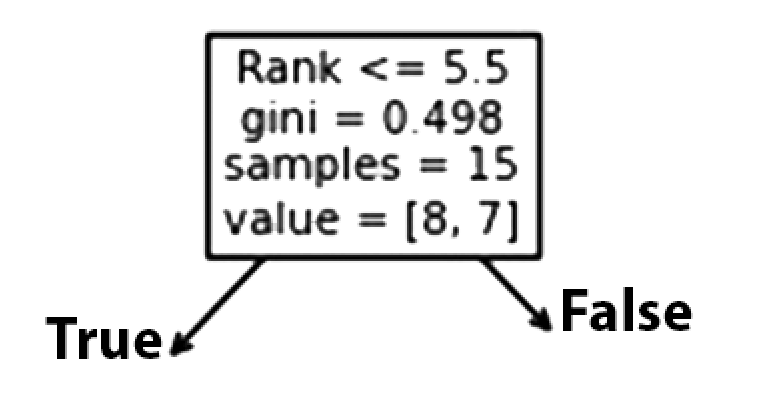
Rank
A singer with a Rank of 5.5 or lower will follow the True arrow (to the left), and the rest will follow the False arrow (to the right).
The quality of the split is determined by gini = 0.498, which is always a number between 0.0 and 0.5, where 0.0 indicates that all samples received the same answer, while 0.5 indicates that it is centered.
Considering this is the first step in the selection process, there are 15 singers left at this point.
This value indicates that out of these 15 singers, 8 will have a “NO”, while 7 will have a “GO”.
Gini
GINI is one method to split the samples, but there are many others. This tutorial demonstrates the GINI method.
Gini’s method uses the following formula:
Gini = 1 - (x/n)2 - (y/n)2Taking x as the number of positive responses (“GO“), n as the number of samples, and y as the number of negative responses (“NO“), the following calculation can be made:
1 - (7 / 13)2 - (6 / 13)2 = 0.497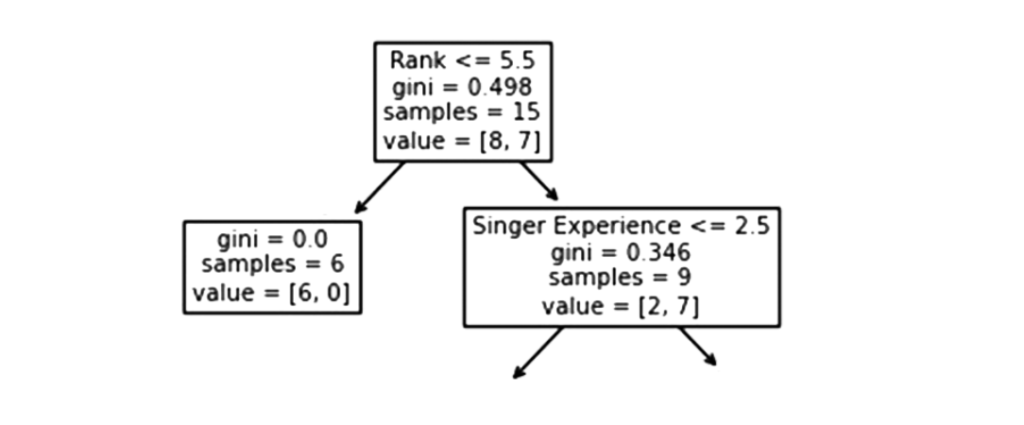
Following that, there are two boxes, one for singers with a ‘Rank‘ of less than 5.5, and one for the remainder.
True – 6 Singers End Here:
A Gini value of 0.0 implies the same result was obtained by all samples.
A sample size of 6 indicates that there are only Six singers left in this branch (6 singers with a Rank of 5.5 or lower).
In this case, 6 will result in a “NO” and 0 will result in a “GO”.
False – 9 Singers Continue:
Singer Experience
In the context of singers experience, a value of less than 2.5 means that singers with a singing experience value that falls under 2.5 years will follow the arrow to the right and the rest will follow the arrow to the left.
The gini value of 0.346 indicates that 34.6% of the samples will go in one direction.
A sample size of 9 indicates that there are 9 singers left in this branch (9 singers with a singing Rank higher than 5.5).
According to value = [2, 7] only two of these nine singers will get a “NO” while the other seven will get a “GO”.
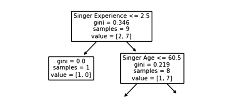
True – 8 Singers Continue:
Singer Age
When the age is 60.5 or less, singers who have reached the age of 60.5 or younger will follow the arrow to the left. Those over the age of 60.5 will follow the arrow to the right.
A Gini value of 0.219 indicates that 21.9% of samples go in a single direction. A sample size of 8 means there are 8 singers left in the branch.
The value of [1, 7] indicates that of these 8 singers, one will get a “NO” and 7 will get a “GO”.
False – One more Singers End Here:
Gini = 0.0 indicates that all samples have the same result.
The sample count of 1 means that there are four singers left in this branch.
The value = [1, 0] indicates that 1 Singers, 1 will receive a “NO” and 0 will receive a “GO“.
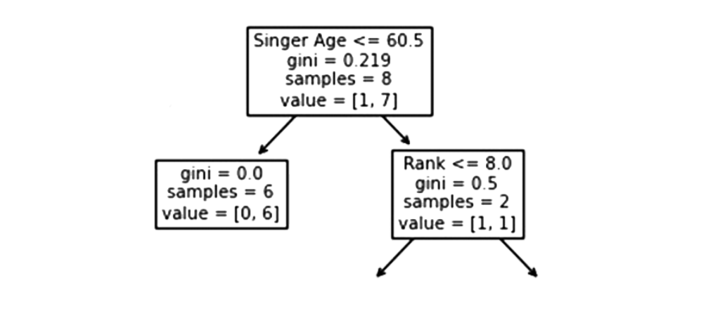
True – 6 Singers End Here:
A Gini value of 0.0 indicates that all samples produced the same result.
The sample size of 6 indicates that there are Six singers left in this branch (6 singers under the age of 60.5).
The value of [0, 6] means that of these 6 singers, 0 will receive a “NO” and 6 will receive a “GO“.
False – 2 Singers Continue:
Rank
Singers with 8.0 or less of rank will follow the arrow to the left, while everyone else will follow the arrow to the right.
Gini = 0.5 indicates that 50% of the samples will go in one direction.
The sample value of 2 indicates that there are two singers left in this branch (2 singers older than 60.5 years).
In this case, the value of [1, 1] indicates that of the 2 singers, one will receive a “NO” and the other will receive a “GO“.
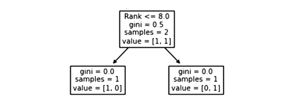
False – 1 Singer Ends Here:
A Gini value of 0.0 implies the same result was obtained by all samples.
The number of samples = 1 indicates that there is only one singer left in this branch (with Rank above 8.0).
The value [1, 0] means that 1 gets a “NO” and 0 gets a “GO“.
True – 1 Singer Ends Here:
A Gini value of 0.0 implies the same result was obtained by all samples.
As of right now, there is only one singer left in this branch (1 singer with 8.0 Rank or lower).
The value of [0, 1] indicates that 0 gets a “NO” and 1 gets a “GO”.
Predict Values
A Decision Tree is useful for predicting new values.
Can you recommend a concert featuring a 35-year-old American singer, who has 12 years of singing experience and a 9 on the singing rank scale?
To predict new values, use the predict() method:
Example
In the case of a 5 singing rank, what would be the answer?
Example
Different Results
After running the Decision Tree enough times, you will see that even the same data feeds it different results.
Because of the Decision Tree, we cannot be 100% certain of the answer since it does not give us a 100% certainty. Based on the probability of an outcome, and the answer will differ depending on the probability of that outcome.
Decision Tree Advantages and Disadvantages
Decision Tree Advantages:
- A decision tree can generate rules that are easy to understand.
- In decision trees, classification is performed without a great deal of computation.
- Both continuous and categorical variables can be handled by decision trees.
- Predictability and classification can be improved by using decision trees.
Decision Tree Disadvantages:
- When estimating continuous attributes, decision trees are less appropriate.
- The use of decision trees can lead to errors when there are many classes and a limited number of training examples when dealing with classification problems.
- Training a decision tree can be computationally expensive. Growing a decision tree is computationally intensive. To find the best split at each node, each candidate splitting field must be sorted.