Numpy Random Poisson Distribution
The NumPy random Poisson function generates random numbers following a Poisson distribution. In this article, we will examine what Poisson distribution is and how to use the NumPy random Poisson function.
What is a Poisson Distribution?
The Poisson distribution is a discrete probability distribution that expresses the probability of a given number of events occurring in a fixed interval of time or space, assuming that the events are independent and that the average rate of occurrence is constant.
The Poisson distribution is often used to model random occurrences, such as:
- Number of customers who arrive at a store.
- Number of cars that pass through a toll booth.
- Number of phone calls received by a call center.
The Poisson distribution is characterized by a single parameter, which represents the average rate of occurrence of the events.
This parameter is denoted by λ (lambda) and is also equal to the variance of the distribution.
The probability mass function (PMF) of the Poisson distribution is given by:
P(mrX = k) = (e^(-λ) * λ^k) / k!
where mrX is the random variable representing the number of events, k is a non-negative integer, e is the base of the natural logarithm, and k! is the factorial of k.
NumPy Random Poisson Function
A Numpy random poisson function is a discrete distribution and is a part of the NumPy.random module and is used to generate random numbers following a Poisson distribution.
It estimates how many times an event could occur in a certain period of time.
For example, what is the chance that a person will eat four meals a day if he eats three meals daily?
A parameter of this function is the following:
| Parameters | Overview |
| lam | The number of instances or the rate of events, for example. Three in the situation above. |
| size | This is how the array will be arranged when it is retrieved. |
Syntax
numpy.random.poisson(lam=1.0, size=None)
where lam is the expected value of the Poisson distribution, and size is the shape of the output array.
The function returns an array of random integers representing the number of events that occur in a fixed interval of time or space.
The values in the array are generated independently of each other and follow a Poisson distribution with parameter λ.
Let’s look at below examples:
Create a random 1×30 distribution for instance 3:
Example:
Randomly distribute the outcomes of 5 as follows:
Example:
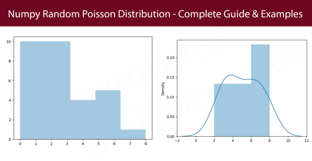
Visualization of Poisson Distribution
To visualize NumPy Random Poisson distribution, we can use Python’s matplotlib library.
We will generate a range of values for the number of occurrences, and then calculate the probability mass function for each value using the Poisson distribution formula.
Finally, we will plot the results as a histogram.
Implementation of visual representation:
Example:
Apply the below code with kde = True:
Example:
Difference Between Normal and Poisson Distribution
In Numpy random poisson, the normal distribution is continuous, while the poisson distribution is discrete.
When the poisson distribution grows wide and long enough, it will become almost identical to the normal distribution with only a few standard deviations and means.
Differences between normal and Poisson distributions can be summarized as follows:
- Normal distribution is used for continuous data, while Poisson distribution is used for count data.
- Normal distribution has two parameters (mean and standard deviation), while Poisson distribution has one parameter (average rate of occurrence).
- Normal distribution is symmetric around the mean, while Poisson distribution is skewed to the right if the average rate of occurrence is small.
- Normal distribution has a continuous probability density function, while Poisson distribution has a discrete probability mass function.
- Normal distribution measures the spread of the data using the standard deviation, while Poisson distribution has a fixed variance equal to the average rate of occurrence.
The below two examples will ensure you understand the difference between Normal and Poisson distribution:
Example:
Example:
Difference Between Poisson and Binomial Distribution
A very slight difference is found between the binomial and poisson distributions, and it is that the binomial distribution is applied for discrete tests, while the poisson distribution is utilized for continuous tests.
However, when n is very high and p is close to 0, binomial distribution is almost equal to poisson distribution, so that n + p is approximately identical to lam.
Differences between Poisson and binomial distributions can be summarized as follows:
- Poisson distribution is used for count data, while binomial distribution is used for the number of successes in a fixed number of trials.
- Poisson distribution has one parameter (average rate of occurrence), while binomial distribution has two parameters (probability of success and number of trials).
- Poisson distribution is skewed to the right if the average rate of occurrence is small, while binomial distribution is symmetric if p=0.5.
- Poisson distribution has a PMF that depends only on the rate parameter, while binomial distribution has a PMF that depends on both the probability of success and the number of trials.
- Poisson distribution is used to approximate the binomial distribution when the number of trials is large and the probability of success is small.
Here are two examples that demonstrate the distinction between the Poisson and Binomial distributions:
Example:
Example:
Conclusion
The NumPy random Poisson function is useful for generating random numbers following a Poisson distribution.
It can be used in a variety of applications, such as simulating customer arrivals, phone calls, or car accidents.
By understanding the Poisson distribution and how to use the NumPy random Poisson function, we can better analyze and model random occurrences in our data.