Quick Guide To Pandas Plotting
We will discuss the advance concepts of Pandas plotting in this article, along with the different types of plots that can be created, as well as how to customize them according to your specifications.
Pandas Plotting
Plot() is the method Pandas implements to generate diagrams.
In Pandas plotting, we can display the diagram on the screen by utilizing Pyplot, a submodule of Matplotlib.
Utilizing Matplotlib, import pyplot and display our empWrong_data.csv DataFrame:
#Here are three lines that allow our compiler capable to draw:
import sys
import matplotlib
matplotlib.use('Agg')
import pandas as pds
import matplotlib.pyplot as pt
mrx_df = pds.read_csv("empWrongdata.csv')
mrx_df.plot()
pt.show()
#To allow our compiler access to draw, we require to insert two lines:
pt.savefig(sys.stdout.buffer)
sys.stdout.flush()
Provide a title and labels for your graph:
#Here are three lines that allow our compiler capable to draw:
import sys
import matplotlib
matplotlib.use('Agg')
import pandas as pds
import matplotlib.pyplot as pt
mrx_df = pds.read_csv("empWrongdata.csv')
mrx_df.plot()
pt.title("MR EXAMPLES", size = 20)
pt.xlabel("Indexes", size = 15)
pt.ylabel("Salaries", size = 15)
pt.show()
#To allow our compiler access to draw, we require to insert two lines:
pt.savefig(sys.stdout.buffer)
sys.stdout.flush()
It can be seen that the examples in this page are based on a CSV file named: empWrong_data.csv.
Download empWrong_data or
Open empWrong_data
Pandas Scatter Plot
If you are plotting Pandas, indicate that you require a scatter plot with the kind argument:
kind = 'scatter'
It is necessary for a scatter plot to have an x- and a y-axis.
We will utilize the term Indexes for the x-axis and the term Salaries for the y-axis in the example below.
Provide the x and y arguments in the following way: x = ‘EMPLOYEE_NAME’, y = ‘SALARY($)’
#Here are three lines that allow our compiler capable to draw:
import sys
import matplotlib
matplotlib.use('Agg')
import pandas as pds
import matplotlib.pyplot as pt
mrx_df = pds.read_csv('empWrongdata.csv')
mrx_df[['EMPLOYEE_NAME','SALARY($)']].plot(kind='scatter', x = "EMPLOYEE_NAME", y = "SALARY($)", color = "blue")
pt.title("EMPLOYEE DATA", size = 15)
pt.show()
#To allow our compiler access to draw, we require to insert two lines:
pt.savefig(sys.stdout.buffer)
sys.stdout.flush()
In the following example modify the colors of the x and y axis labels:
#Here are three lines that allow our compiler capable to draw:
import sys
import matplotlib
matplotlib.use('Agg')
import pandas as pds
import matplotlib.pyplot as pt
mrx_df = pds.read_csv('empWrongdata.csv')
mrx_ax = mrx_df[['EMPLOYEE_NAME', 'SALARY($)']].plot.scatter(x='EMPLOYEE_NAME', y='SALARY($)', color = 'blue')
mrx_ax.set_xlabel('Names', size = 15)
mrx_ax.set_ylabel('Salaries', size = 15)
#Change the x-axis label color
mrx_ax.xaxis.label.set_color('maroon')
#Change the y-axis label color
mrx_ax.yaxis.label.set_color('purple')
pt.title("EMPLOYEE DATA", size = 17)
pt.show()
#To allow our compiler access to draw, we require to insert two lines:
pt.savefig(sys.stdout.buffer)
sys.stdout.flush()
Remember: According to the previous example, we observed that each employee’s salary is efficiently visualized by the scatter plot graph. This is because each name in x axis points out its salary in y axis.
In the next scatterplot, we will place the ID of the employee on the x-axis and the salary information on the y-axis, and then check the relationship:
#Here are three lines that allow our compiler capable to draw:
import sys
import matplotlib
matplotlib.use('Agg')
import pandas as pds
import matplotlib.pyplot as pt
mrx_df = pds.read_csv('empWrongdata.csv')
mrx_df[['EMPLOYEE_ID','SALARY($)']].plot(kind='scatter', x = "EMPLOYEE_ID", y = "SALARY($)", color = "green")
pt.title("EMPLOYEE DATA", size = 15)
pt.show()
#To allow our compiler access to draw, we require to insert two lines:
pt.savefig(sys.stdout.buffer)
sys.stdout.flush()
Apply some styling on the following scatter plotting:
#Here are three lines that allow our compiler capable to draw:
import sys
import matplotlib
matplotlib.use('Agg')
import pandas as pds
import matplotlib.pyplot as pt
matplotlib.style.use('dark_background')
mrx_df = pds.read_csv('empWrongdata.csv')
mrx_df[['EMPLOYEE_ID','SALARY($)']].plot(kind='scatter', x = "EMPLOYEE_ID", y = "SALARY($)", color = "yellow", s = 200)
pt.title("EMPLOYEE DATA", size = 20, color = 'snow')
pt.xticks(fontsize = 15)
pt.yticks(fontsize = 15)
pt.xlabel("EMPLOYEE_ID" ,fontsize=17, color = 'deepskyblue')
pt.ylabel("SALARY($)" ,fontsize=17, color = 'deepskyblue')
pt.show()
#To allow our compiler access to draw, we require to insert two lines:
pt.savefig(sys.stdout.buffer)
sys.stdout.flush()
Pandas Plotting Histogram
It is possible to tell the program that you want a histogram by providing the kind argument:
kind = 'hist'
Histograms require only one column.
In a histogram, we can see the frequency of each interval, for example, Four customers are waiting between 1 and 45 seconds.
The following example utilizes the SALARY($) column to generate the histogram:
#Here are three lines that allow our compiler capable to draw:
import sys
import matplotlib
matplotlib.use('Agg')
import pandas as pds
import matplotlib.pyplot as pt
matplotlib.style.use('Solarize_Light2')
mrx_df = pds.read_csv('empWrongdata.csv')
mrx_df[['EMPLOYEE_ID','SALARY($)']].plot(kind='hist', x = "EMPLOYEE_ID", y = "SALARY($)", color = "yellow",bins = 40)
pt.title("EMPLOYEE DATA", size = 20, color = 'black', fontweight='bold')
pt.xticks(fontsize = 15)
pt.yticks(fontsize = 15)
pt.xlabel("SALARY($)" ,fontsize=17, color = 'deepskyblue', fontweight='bold')
pt.ylabel("SALARY($)" ,fontsize=17, color = 'deepskyblue', fontweight='bold')
pt.show()
#To allow our compiler access to draw, we require to insert two lines:
pt.savefig(sys.stdout.buffer)
sys.stdout.flush()
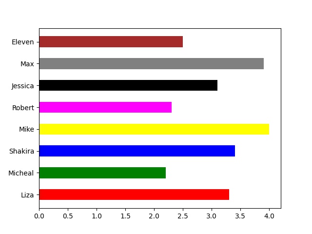
Apply the edge color and set the line width to the following histogram:
#Here are three lines that allow our compiler capable to draw:
import sys
import matplotlib
matplotlib.use('Agg')
import pandas as pds
import matplotlib.pyplot as pt
matplotlib.style.use('Solarize_Light2')
mrx_df = pds.read_csv('empWrongdata.csv')
mrx_df[['EMPLOYEE_NAME','SALARY($)']].plot(kind='hist', x = "EMPLOYEE_NAME", y = "SALARY($)", color = "blue", bins = 15, edgecolor = 'orange', linewidth = 5)
pt.title("EMPLOYEE DATA", size = 20, color = 'black', fontweight='bold')
pt.xticks(fontsize = 15)
pt.yticks(fontsize = 15)
pt.xlabel("SALARY($)" ,fontsize=17, color = 'deepskyblue', fontweight='bold')
pt.ylabel("EMPLOYEES" ,fontsize=17, color = 'deepskyblue', fontweight='bold')
pt.show()
#To allow our compiler access to draw, we require to insert two lines:
pt.savefig(sys.stdout.buffer)
sys.stdout.flush()
Reminder: According to Pandas plotting, the histogram shows us that some employees in a company had the same salary ratio and some employees had different salaries.
Example Explanation
The above example code reads in data from a CSV file, creates a histogram of the salaries of the employees using the plot() function from the Pandas library, and customizes the plot using various functions from the Matplotlib library.
The matplotlib.use(‘Agg’) line is used to set the Matplotlib backend to ‘Agg’, which allows for plotting without a display. The sys and matplotlib libraries are then imported, and the style.use() function is used to set the plot style to ‘Solarize_Light2’.
The pds.read_csv() function reads in the data from the CSV file and stores it in a Pandas DataFrame mrx_df. The plot() function is then called on the DataFrame to create a histogram, with the kind parameter set to ‘hist‘ and the x and y parameters set to ‘EMPLOYEE_NAME’ and ‘SALARY($)’, respectively. The color parameter sets the color of the histogram bars to blue, bins parameter sets the number of bins to 15, and the edgecolor and linewidth parameters are used to customize the appearance of the histogram.
Finally, the plot is customized using various functions from the Matplotlib library. The title() function sets the plot title to ‘EMPLOYEE DATA’, with a font size of 20, black color, and bold font weight. The xticks() and yticks() functions set the font size of the tick labels on the x- and y-axes to 15, respectively. The xlabel() and ylabel() functions are used to set the labels of the x- and y-axes, respectively, with a font size of 17, deep sky blue color, and bold font weight.
The plot is then displayed using the show() function, and to allow the plot to be saved without a display, the savefig() function is used with the sys.stdout.buffer argument and sys.stdout.flush() function is called.
Pandas Plotting Benefits
There are several benefits for using Pandas plotting:
- Pandas provides a simple and intuitive interface for creating plots. You can create plots using just a few lines of code, which is especially useful for exploratory data analysis.
- Pandas provides a variety of plot types and customization options, allowing you to create a wide range of plots to suit your needs.
- Pandas uses Matplotlib, one of the most popular plotting libraries in Python, as its backend. This means that you can use all of the customization options and features provided by Matplotlib in your Pandas plots.
- Pandas also supports interactive plotting using the plotly and bokeh libraries, allowing you to create interactive visualizations that can be explored in a web browser.
- Pandas integrates well with other data analysis tools in Python, such as NumPy and Scikit-learn, making it easy to analyze and visualize your data in one place.