Binomial Distribution In NumPy
The binomial distribution is a probability distribution that describes the number of successes in a fixed number of independent trials. In this article, we’ll explore Numpy Random binomial distribution and how to use it.
The numpy.random module in Python provides a function for generating random numbers from the Binomial distribution, known as numpy.random.binomial.
Numpy Random Binomial
We can say that Numpy random binomial is a discrete distribution in Numpy random binomial.
As an outcome, it explains the conclusion of binary scenarios, e.g. tossing a coin and it will either come up heads or tails, etc.
Syntax
numpy.random.binomial(n, p, size=None)
There are three parameters that make up this function:
| Parameters | Overview |
| n | the number of tests that have been conducted. |
| p | Probability of each event happening (e.g. for tossing a coin, there is a probability of 0.5 for each). |
| size | This parameter specifies the shape of the array that will be generated. |
Discrete Distribution
As an example, a coin toss’s outcome is discrete because it can only be heads or tails, while the height of people is continuous because it can be 160, 160.1, 160.11, etc.
Utilizing 5 attempts for the coin toss, we can collect 8 data points:
Example:
Based on four trials of coin toss, produce two data points:
Example:
Binomial Distribution Visualization
Implementation:
Example:
Implement the following example with True kernel density estimation:
Example:
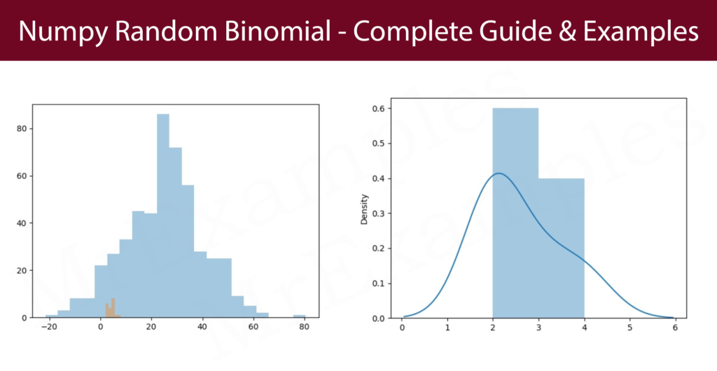
Difference Between Normal and Binomial Distribution
According to Numpy random binomial, the primary difference is that normal distribution is continuous, while binomial is discrete, but if there are sufficient data points it will be almost identical to normal distribution.
Here is the code to run:
Example:
Implement the following example with hist = True and kde = False.
Example:
Conclusion
In this article, we discussed the numpy random binomial distribution in detail, including its definition, parameters, and how to use it.
We also showed how to visualize the Binomial distribution using a histogram.