Linear Regression In Python Machine Learning
Our educational goal today is to expand our knowledge concerning Python Ml linear regression with examples.
What Is Regression?
When you are looking for a relationship between variables, you use the term regression.
This relationship is used in Machine Learning and in statistical modeling to forecast future happenings.
Linear Regression In Python
A linear regression algorithm is a machine learning algorithm based on supervised learning – the program performs a regression analysis.
A regression model predicts a target value based on independent variables. Forecasting is mainly determined by how variables relate to each other.
Dependent and independent variables are considered differently in different regression models, and so is the number of independent variables.
Many names can refer to a regression’s dependent variable.
Variables may be called outcome variables, criterion variables, endogenous variables, or regressions.
Exogenous variables can be regressors, predictor variables, or predictor variables.
The linear regression process draws a straight line through all data points based on their relationship.
Future values can be predicted using this line.
A very important aspect of Machine Learning is the ability to predict the future.
How Does Linear Regression Works?
The Python language allows users to find relationships between data points and to draw lines of linear regression. Let us show you how
It is easier to use these methods than to work through mathematical formulas.
Firms are represented by the x-axis, and performance is represented by the y-axis in the example below.
18 firms have been registered and their performance assessed as they pass a tollbooth. Here is a linear regression test we can do with the data we collected:
Linear Regression Example Image:
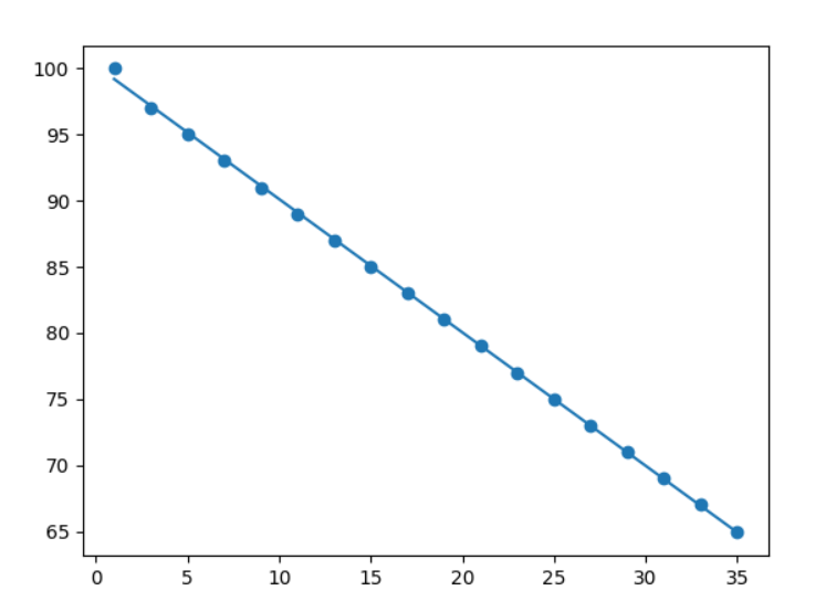
Drawing a scatter plot is the first step:
Example
You can import Scipy and draw a linear regression line as follows:
Example
Result:
Explanation of the example
You will be required to import the modules you need.
The Matplotlib and SciPy modules are covered in our Matplotlib and SciPy posts.
import matplotlib.pyplot as plt
from scipy
import stats
The x and y axis values should be represented by arrays – We have used mrx as x and ample for y axis as follows:
mrx = [1,3,5,7,9,11,13,15,17,19,21,23,25,27,29,31,33,35]
ample = [99,97,95,93,91,89,87,85,83,81,79,77,75,73,71,69,67,65]
Perform a linear regression method that returns some significant key values:
slope, intercept, r,
p, std_err = stats.linregress(mrx, ample)
Make a function that returns a new value based on slope and intercept.
A new value represents the location of the corresponding x value on the y-axis:
def pymlfunc(mrx):
return slope * mrx + intercept
The function should be run for each value in the mrx array. As a result, a new array will be created with new values for the y-axis:
firms = list(map(pymlfunc, mrx))
Create the original scatter plot by drawing the following:
plt.scatter(mrx, ample)
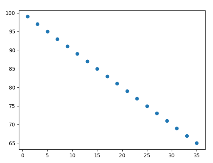
Using the linear regression equation, draw a line:
plt.plot(mrx, firms)
Finally, display the diagram as follows:
plt.show()
R – Relationship
Linear regression cannot be used to predict anything if there is no relationship between the values of the x-axis and the values of the y-axis.
Correlation coefficients, such as r, are used to measure this relationship.
A r value of -1 to 1 indicates that there is no relationship, while a 1 (or -1) indicates 100% relatedness.
You only need to supply Python and the Scipy module with the mrx and ample variable values to calculate this value.
Does my linear regression model fit my data well?
Example
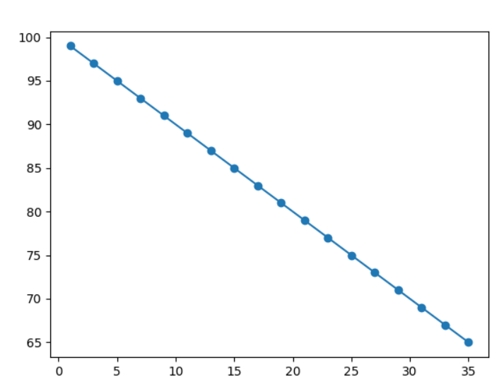
The result -1.0 indicates that there is a 100% relationship, and it indicates that linear regression could be used in the future to make predictions.
Predict Future
Our collected data can now be examined to predict future values.
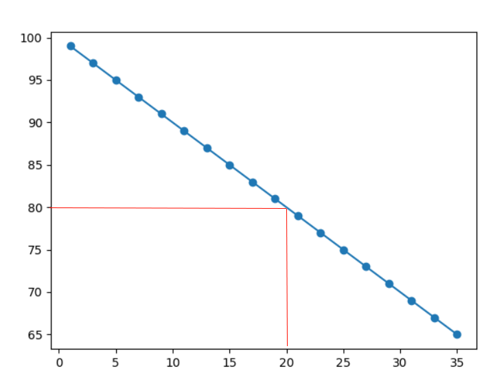
Consider a company that is 20 years old and try to predict its performance.
Using the pymlfunc() function from the previous example, we can achieve this:
def pymlfunc(mrx):
return slope * mrx + intercept
A firm that is 20 years old will perform as follows:
Example
As we can see from the diagram, the example predicted a performance of 80:
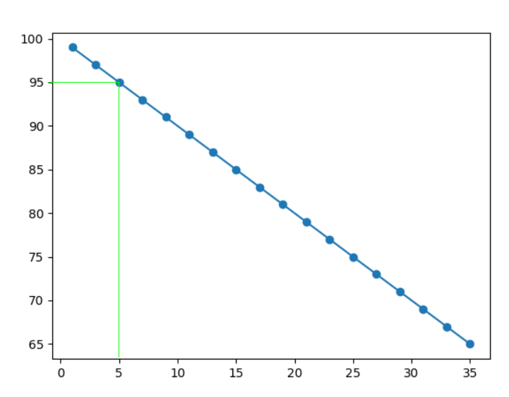
The performance of a five-year-old company is now predicted:
A firm that is just 5 years old will perform as follows:
Example
This example predicted a 95% performance, as can be seen in the diagram below:
Based on our prediction, we found that the new firms grew much faster than the old companies.
Bad Fit?
Here is an example where linear regression may not be the best form of prediction when it comes to predicting future values.
Linear regression should be very poorly fitted with these values for the x-axes and y-axes:
Example
Result:

How about the r for relationship?
An extremely low r value should be obtained.
Example
According to the results, 0.0364 represents a very bad relationship between the two variables and shows us that the data set may not be suitable for linear regression using this method.